


本文为美国南卡罗莱纳医科大学神经科学系/昌平实验室脑科学与类脑研究部/北京大学生物医学前沿创新中心 刘河生 教授团队发 Science Advances 的工作,题为“Robust dynamic brain coactivation states estimated in individuals”。DOI:10.1126/sciadv.abq8566。
Abstract
大量证据表明,大脑功能连接并非静态,而是动态的。捕捉个体大脑中的瞬时网络交互需要一种具有足够个体内可靠性的技术。本文介绍了一种基于个体化网络的动态分析技术,并证明其在检测个体特定的大脑状态方面具有可靠性,无论是在静息状态还是在具有认知挑战的语言任务中。我们评估了大脑状态在半球不对称性方面的表现,以及各种表型因素(如利手和性别)如何影响网络动态,发现了一种右偏侧化的大脑状态,该状态在男性和右利手个体中更为常见。我们还展示了42名皮质下卒中患者在6个月内的纵向大脑状态变化。我们的方法能够量化个体特定的动态大脑状态,并具有在基础和临床神经科学研究中应用的潜力。
Introduction
跨多个空间和时间尺度的信息协调是大脑最佳功能的前提,涵盖了认知和行为领域。分层组织的电生理振荡的同步促进了局部和分布式大脑区域的动态整合,并使得快速高效的皮质处理所需的连贯功能网络配置得以形成和解体。控制大规模网络动态的组织原则,这些动态在空间分布和功能分化的皮质区域上表现出时间变化和内在耦合活动,目前才刚刚开始被理解。来自多种模态的新证据表明,功能状态模式是动态形成或表达的。这些瞬态网络配置及其在精细时间尺度上出现的时空动态不仅在所谓的“静息态”中被观察到,还在各种认知任务中被观察到。静息态功能磁共振成像(fMRI)标准分析策略的新扩展表明,区域之间的功能耦合在整个标准扫描过程中并非静态,而是高度动态的。除了早期证据表明可能与行为、生理、意识状态、结构和电生理相关外,动态功能连接(FC)方法还揭示了缓慢波动且可重复的全脑配置,这些配置在跨时间点平均时会丢失。最近的分析技术进步使得血氧水平依赖(BOLD)MR图像可以分解为潜在的时间变化大脑共激活模式,这些模式共同形成了典型大规模内在网络(如默认网络(DN)和背侧注意网络)的平均FC图。对单体积MR图像的检查,而不是在窗口期内平均,能够检测到在更小时间尺度上发生的瞬态功能网络交互,从而更好地评估其时间依赖性。基于单体积的分析不受影响二阶统计的“采样变异性”的混淆,例如滑动窗口中的时间相关性。因此,这种方法可能特别适用于研究跨空间不同和功能分化的大脑区域的网络动态。然而,这种方法主要应用于研究组水平的大脑特征,尚未在个体水平上表现出足够的可靠性。更广泛地说,fMRI研究整体上面临着个体水平可靠性低的挑战,这阻碍了fMRI的临床应用和有意义的神经影像生物标志物的发现。尽管先前的研究表明,通过增加扫描长度可以提高某些fMRI测量的可靠性,但尚不清楚动态指标(尤其是基于单体积图像的指标)是否也能从更长的扫描中受益。
在这里,我们引入了一种“基于个体化网络的单帧共激活模式估计”(Individualized Network-based Singleframe Coactivation Pattern Estimation,INSCAPE)方法,以探索个体水平上动态大脑状态网络配置的时空特征。本研究的目标是可靠地表征个体特定的功能特性,并捕捉功能大脑状态时空动态中的个体差异。作为测试,我们研究了功能偏侧化,这是人类大脑组织的一个经过充分研究的基本特性,并且具有高度个体特异性。我们探讨了通过我们的INSCAPE方法识别的功能大脑状态的时空动态在多大程度上表现出语言处理的半球不对称性。鉴于语言功能偏侧化与利手和性别之间的联系,我们还研究了这些表型特征是否与偏侧化大脑状态的发生有关。最后,为了展示该技术在未来患者相关研究中的潜力,我们研究了42名皮质下卒中患者在6个月内的纵向大脑状态网络动态变化,以跟踪卒中后恢复的时间进程和时空特性。
Materials and Methods
Experimental design
本研究包括了七个fMRI数据集,涉及超过1000名受试者和2000多次扫描。请注意,数据集I、III、IV和V均来自脑基因组超结构项目(GSP)。数据集III、IV和V部分与数据集I重叠。详情如下。(数据集基础信息如下,更多细节及扫描参数见原文)
Dataset I
The first dataset consisted of 1000 healthy, young adult participants (mean age 21.3 ± 3.1 years; 427 males) from the GSP. Each subject performed one or two restingstate fMRI runs (6 min 12 s per run) and a structural run. Participants were instructed to stay awake and keep eyes open during the resting-state scans.
Dataset II
The second dataset included 30 healthy, young adults (mean age 24 ± 2.4 years; 15 males) that were collected as part of the CoRRHNU. Each participant underwent 10 resting-state fMRI scans (10 min per scan) and a structural MRI scan across a period of 1 month.Participants were instructed to keep their eyes open and relax during the resting-state fMRI scans.
Dataset III
The third dataset comprised a subset of subjects from the GSP dataset (i.e., Dataset I) and contained 55 young, healthy adult articipants (mean age 21.1 ± 2.7 years; 25 males). Each participant underwent two resting-state fMRI runs (6 min 12 s per run) and two task-based fMRI runs (6 min 12 s per run) wherein a semantic classification language task was performed.
Dataset IV
The fourth dataset consisted of 52 left-handed and 52 right-handed subjects matched by age, gender,ethnicity, education, fMRI data acquisition, and data quality that were acquired as part of the GSP. For each participant, two resting-state fMRI runs (6 min 12 s per run) and a structural MRI run were acquired.
Dataset V
The fifth dataset was a subset of the GSP dataset (Dataset I) and consisted of 279 male and 279 female participants matched by age, education, and handedness. For each participant, one or two restingstate fMRI runs (6 min 12 s per run) were acquired along with a structural T1-weighted scan.
Dataset VI
The sixth dataset included 42 patients with first-episode subcortical stroke (mean age 50.7 ± 11.8 years; 39 males) and 23 age-matched healthy control participants (mean age 51.8 ± 6.9 years; 9 males).Each participant underwent five resting-state fMRI scans over a period of 6 months (at 1 to 7, 14, 30, 90, and 180 days after stroke). Each scan session consisted of two to four resting-state fMRI runs (6 min per run) and a structural MRI run.Participants were instructed to stay awake and keep their eyes open during the resting-state scans.
Dataset VII
The seventh dataset included 100 young healthy individuals (the “Unrelated 100” group, age between 22 and 35 except one individual from the 36+ group, 54 females) made publicly available by the HCP, supported by the WU-Minn Consortium. Each subject had two resting-state fMRI sessions (each session consisted of one run with left-to-right direction phase encoding and one run with right-to-left direction, 14 min 24 s per run).
Data preprocessing
fMRI数据使用先前描述的分析流程进行预处理,包括以下步骤:(i)时间层校正;(ii)头部运动的刚体校正;(iii)全局平均信号强度归一化;(iv)带通滤波(0.01-0.08 Hz),以及(v)头部运动参数和全脑、脑室和白质信号的回归。
结构数据使用FreeSurfer v5.3.0软件包进行预处理。对于每位受试者,从结构T1加权图像重建皮质表面网格,然后注册到共同的球形坐标系。预处理后的功能数据随后注册到FreeSurfer“fsaverage6”皮质表面模板,每个半球包含40,962个顶点。在表面空间中使用6 mm 全宽半高高斯核进行空间平滑。为了减少计算成本,平滑后的数据随后下采样到“fsaverage4”模板,每个半球包含2562个顶点。
Network-based single-frame dynamic coactivation analysis
INSCAPE方法包括以下两个步骤,详细描述如下并如 Fig.1 所示:(i)生成脑共激活状态的组水平模板,(ii)估计个体特异性脑状态。
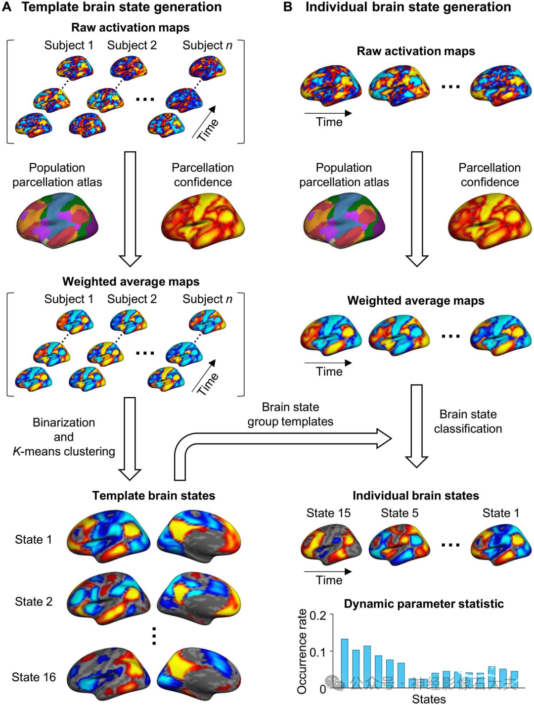
Fig. 1. Schematic of the INSCAPE approach. (A) The group templates of brain coactivation states were generated using a resting-state fMRI dataset containing 846 healthy subjects from the GSP (Dataset I). Specifically, the preprocessed fMRI data of each subject were projected to the FreeSurfer fsaverage4 surface space, which has 2562 vertices per hemisphere. For each time frame of BOLD data, the raw activation map was weighted by the parcellation confidence derived from a populationbased cortical parcellation and averaged within each of the 48 network patches (24 per hemisphere). The mean activations of the 48 patches were then binarized (i.e.,values larger than 0 were set to 1 and values smaller than 0 were set to -1) to represent the mean weighted coactivation maps that were then concatenated along with the time series across all subjects. A k-means clustering analysis was then performed to classify the fMRI frames into 16 clusters. The optimal cluster number of 16 was selected on the basis of results from the test-retest reliability analysis (see fig. S1) because it balanced the test-retest reliability with the diversity of the brain states. Last, the maps of fMRI frames assigned to the same cluster were averaged to generate the group templates for the 16 dynamic brain states. (B) At an individual subject level, the maps of the preprocessed fMRI data were first weighted by the parcellation confidence and averaged within the 48 patches using the same procedure described above for group template generation. Each patch map was then assigned to one of the 16 template brain states having the shortest spatial distance to it. The occurrence rate of each brain state was calculated as the percentage of frames assigned to a given brain state out of the total number of frames.
Generating group template of brain states
我们使用数据集I生成共激活脑状态的组水平模板。由于头部运动可能混淆BOLD信号,我们仅纳入头部运动较低的受试者,定义为平均和最大头部运动(帧间位移)分别低于0.1 mm 和 0.5 mm。在GSP数据集的1000名受试者中,154名受试者不符合这些标准,因此被排除在后续分析之外,最终样本为846名受试者。这一严格的头部运动控制标准仅用于创建模板脑状态,确保模板受头部运动相关噪声的影响最小。我们在其他数据集的后续分析中未基于头部运动排除数据。生成动态共激活脑状态组模板的过程如 Fig.1A 所示。首先,创建了一个基于网络的权重字典,以抑制噪声的影响并保留原始共激活数据的内在网络结构。具体来说,为了生成这个权重字典,将来自基于人群的皮质分区的七个典型功能网络图谱划分为多个不连续的补丁。保留在左右半球中均表示的补丁,最终得到48个网络补丁(每半球24个补丁)。然后提取这48个网络补丁的分区置信度,组成网络权重字典。分区置信度指的是在基于人群的皮质分区过程中,每个顶点被分配到特定功能网络的概率。位于网络补丁中心的顶点通常比靠近网络边界的顶点具有更高的分区置信度。创建权重字典后,对每个时间点的每个顶点的预处理fMRI数据进行加权。加权的单帧fMRI数据随后在每个网络补丁内平均,并二值化,使得大于0的值设为1,小于0的值设为-1。所有受试者的二值化fMRI数据沿其时间序列连接,并使用k均值聚类分析将其分类为16个团块或脑状态。根据结果脑状态的受试者内测试-重测可靠性选择此簇数(见 fig. S1)。最后,将每个簇的图在受试者间平均,组成每个脑状态的组模板。
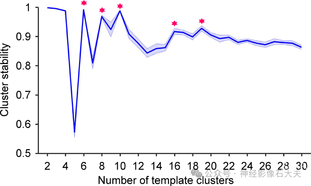
Fig. S1.Determination of the optimal cluster number based on test-retest stability of brain states. Withinsubject test-retest stability of the clustering algorithm was used to optimize the number of brain states. Half of the resting-state runs were randomly selected from each of the 846 subjects from Dataset I and assigned to the test group, with the other half assigned to the retest group. The stability of the clustering analysis was estimated as the mean spatial similarity of brain states derived from the test and retest groups. This test-retest procedure was repeated 100 times. Mean stability (dark blue curve) and ±SEM (blue shadowed areas) across the 100 repetitions are plotted. Several local maxima on the curve were identified (marked with red stars), suggesting that solutions of 6, 8, 10, 16, and 19 clusters were relatively stable. In this study, we selected 16 clusters for further analyses since it balanced the test-retest reliability with the diversity of the brain states.
Estimating individual-specific brain states
在个体水平上,首先按照上述相同程序(Fig.1A)对每位受试者的功能图像进行加权。然后将每个时间帧的加权图与脑状态的组模板进行比较,并将其分配给空间距离最短的脑状态。需要注意的是,在个体水平上,图像未进行二值化。分配给同一脑状态的功能图像进行平均,得到个体化的脑状态图(Fig.1B)。对于16个脑状态中的每一个,状态发生率量化为给定脑状态的时间帧数除以fMRI总时间帧数。
Evaluating the reliability of INSCAPE analysis
使用来自CoRR-HNU数据集(数据集II)的30名年轻健康受试者的独立样本评估INSCAPE方法的测试-重测可靠性。每位受试者进行了10次独立的10分钟静息态fMRI扫描。前五次扫描分配给测试会话,后五次扫描分配给重测会话(每个会话50分钟)。然后,估计测试和重测会话中16个脑状态的发生率。使用每位受试者内16个脑状态发生率的相似性(皮尔逊相关系数)评估INSCAPE分析的受试者内可靠性。使用任何两名受试者之间估计的发生率相似性评估受试者间相似性。鉴于数据长度对动态分析结果的影响,我们还通过计算10种不同测试-重测数据长度(从5分钟到50分钟,每次增加5分钟)的脑状态发生率的可靠性来量化 INSCAPE 结果的测试-重测可靠性。
Estimating functional lateralization of brain states
为了探索共激活脑状态的功能偏侧化程度,首先将来自GSP数据集的16个脑状态的平均图(即组模板)注册到FreeSurfer对称皮质表面模板,每半球包含2562个顶点。对于每个脑状态,计算左右半球中具有正激活值的顶点数。然后按以下公式计算给定脑状态的偏侧化指数(LI):

其中 ![]() 是左半球中正激活的顶点数,
是左半球中正激活的顶点数,![]() 是右半球中正激活的顶点数,
是右半球中正激活的顶点数,![]() 是单个半球中的总顶点数(2562个顶点)。需要注意的是,此LI是在组模板而非个体水平上评估的。正LI值表示左偏侧化,负LI值表示右偏侧化。此外,为了验证皮质上共激活脑状态的功能偏侧化是否也能在小脑中观察到,我们在MNI152体积空间的小脑掩模内计算了平均共激活图。
是单个半球中的总顶点数(2562个顶点)。需要注意的是,此LI是在组模板而非个体水平上评估的。正LI值表示左偏侧化,负LI值表示右偏侧化。此外,为了验证皮质上共激活脑状态的功能偏侧化是否也能在小脑中观察到,我们在MNI152体积空间的小脑掩模内计算了平均共激活图。
功能偏侧化是人类大脑的一个基本属性,也与利手性和性别有关。在这里,我们研究了通过INSCAPE方法识别的脑状态是否能反映功能偏侧化,以及它们是否显示出与利手和性别相关的差异。首先估计了55名健康受试者(数据集III)在语言任务(即语义决策任务)和静息态期间扫描的偏侧化脑状态的发生率。使用一系列配对样本t检验来检查16个共激活脑状态的发生率在任务驱动和静息态条件下是否显著不同。然后根据两半球的不对称激活,使用先前报告的方法计算每位受试者的语言LI。计算语言LI与任务期间最左偏侧化脑状态发生率之间的相关性。在语言任务期间,计算所有受试者在每个时间帧中最左偏侧化和最右偏侧化脑状态的发生率,然后按受试者数归一化。为了研究偏侧化脑状态的发生是否与语言相关处理有关,我们使用皮尔逊相关将16个共激活脑状态的归一化发生率与语言任务起始引起的血流动力学响应曲线进行比较。
此外,为了确定利手对脑状态功能偏侧化的影响,计算了52名左撇子和52名人口统计学匹配的右撇子受试者(数据集IV)的脑状态发生率。使用配对样本t检验来检查脑状态发生率的差异是否受利手影响。我们还使用Kolmogorov-Smirnov检验比较了左撇子和右撇子受试者的发生率分布。在另一个数据集(数据集V;按年龄、教育程度和利手性匹配的279名男性和279名女性)中进行了相同的分析,以检查性别是否影响偏侧化脑状态的发生。
Tracking longitudinal changes in the occurrence rates of brain states during the poststroke recovery period
我们量化了42名皮质下卒中患者在卒中后五个时间点(即卒中后1至7天、14天、30天、90天和180天)和23名健康对照受试者(数据集VI)的脑状态发生率。将第一次扫描会话(作为基线扫描,卒中后1至7天内采集)与卒中后14天、30天、90天和180天的四次后续扫描会话的发生率进行比较。使用重复测量ANOVA来研究脑状态发生率在6个月卒中后恢复期间相对于基线时间点的变化。我们将时间(第7天、14天、30天、90天和180天)指定为受试者内因素,受试者为固定因素。使用配对样本t检验进行一系列事后分析,以确定哪些时间点的发生率与基线时间点显著不同。我们还使用双样本t检验比较了患者组和健康对照组的发生率,以确定患者在6个月卒中后恢复期间动态脑状态的发生率是否恢复到对照组水平。
Statistical analysis
通过计算发现数据集和复制数据集中16个脑状态发生率的皮尔逊相关性来评估INSCAPE方法的可重复性。脑状态图的空间相似性通过斯皮尔曼相关性量化。应用Durbin-Watson检验来检查相邻顶点之间的空间依赖性对相关性的潜在影响。具体来说,我们对7%的顶点进行重复(n = 1000)随机抽样,并在顶点子集上计算相关系数。Durbin-Watson检验用于计算每个子集的空间依赖性,并在1000次迭代中取平均值。在本研究空间相关报告中,Durbin-Watson统计量的值接近2,P > 0.05,表明顶点子集中没有显著的空间自相关性。使用双样本t检验检查受试者内和受试者间状态发生率相似性之间的差异。使用配对t检验评估语言任务期间状态发生率与静息态相比的变化。使用皮尔逊相关研究任务驱动的语言LI与左偏侧化状态发生率之间的关系,以及语言任务期间所有受试者在每个时间点的脑状态发生率与任务处理引起的血流动力学响应曲线之间的关系。使用配对t检验比较左撇子和右撇子以及男性和女性受试者之间状态发生率的差异。使用Kolmogorov-Smirnov检验比较利手和性别中发生率的分布。对于卒中患者数据,使用重复测量ANOVA评估卒中后恢复期间脑状态发生率的变化。使用配对t检验确定哪些时间点的发生率与基线时间点显著不同。
Results
Different brain states have specific coactivation patterns and occurrence rates
使用来自脑基因组超结构项目(GSP;数据集I)的846名健康个体的静息态fMRI数据,通过INSCAPE方法生成了16个大脑状态的组水平模板(见 Fig.1和 Materials and Methods)。大脑状态的数量根据测试-重测可靠性结果选择(见 fig.S1)。然后估计所有大脑状态的发生率,并按降序排列(Fig.2)。通过将分配到同一大脑状态的fMRI帧平均计算平均共激活图,并显示在膨胀的皮质表面上。所有大脑状态的共激活模式都表现出内在的功能网络特性。具有默认网络(DN)激活的大脑状态在静息状态下的发生率最高,其次是表现出突显网络(SN)和额顶控制网络(FPN)区域共激活的大脑状态。此外,还识别出属于其他网络(如腹侧注意网络、视觉网络和感觉运动网络)的不同共激活大脑区域组合。值得注意的是,我们观察到特定的大脑状态显示出半球偏侧化,并在下一节中详细讨论这些结果。
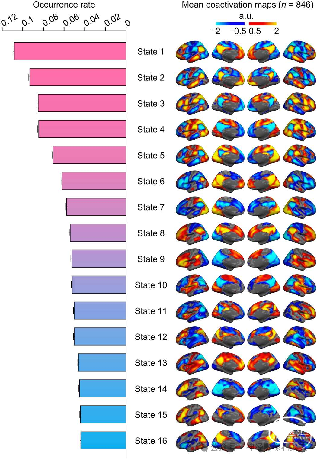
Fig. 2. Occurrence rate and spatial maps of the 16 coactivated brain states. The group templates of brain coactivation states were computed using the INSCAPE approach across 846 healthy individuals from the GSP dataset. The group-level brain state coactivation maps were generated by averaging the fMRI time frames assigned to the same cluster across subjects and ranking them by their rate of occurrence in descending order. Of the 16 brains states, states 1 through 4 showed canonical DN activation and had the highest occurrence rates across subjects during resting state. a.u., arbitrary units.
为了验证大脑状态的可重复性,我们在GSP数据集(数据集I)的一半中计算了大脑状态共激活图及其发生率,这部分数据被指定为发现样本(n = 423),然后在另一半GSP数据集中独立复制了这种方法,这部分数据被指定为复制样本(n = 423)。发现和复制样本中16个大脑状态的发生率高度相关,表明在群体水平上具有高度可重复性(fig.S2;Pearson相关性,r = 0.995,P < 0.001)。16个大脑状态的相应共激活图也表现出高度的空间相似性(平均空间相似性±SD,r = 0.992 ± 0.003,P < 0.001)。
尽管在当前研究中选择了16个大脑状态作为分析的最佳聚类数,因为它在测试-重测可靠性和大脑状态的多样性之间取得了平衡,但我们也研究了10个和19个聚类的解决方案,因为这两个局部最优解决方案在GSP数据集中产生了较高的置换测试-重测可靠性(见 fig.S1)。尽管19个聚类解决方案生成的大脑状态数量多于10个聚类解决方案,但两种解决方案都产生了具有共同时空共激活特征的大脑状态。此外,这些大脑状态的发生率顺序高度相似(fig.S3)。例如,在10个和19个聚类解决方案中,发生率最高的前四个大脑状态的平均共激活图显示出相似的共激活特征。这些发现表明,19个聚类解决方案中的额外大脑状态可能是从10个聚类解决方案中识别的其他大脑状态配置的分解中得出的。
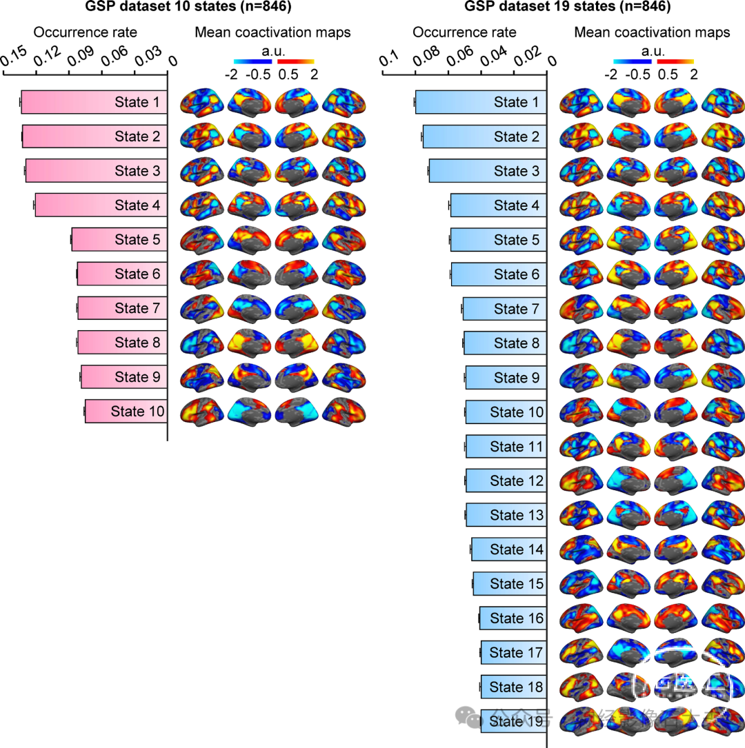
Fig. S3.Characterization of the occurrence rates and mean coactivation maps of brain states derived from the 10- and 19-cluster solutions. The occurrence rate and mean coactivation maps derived from the 10- and 19-cluster solutions were estimated in the GSP dataset (Dataset I; n = 846). Although the 19-cluster solution has more clusters than the 10-cluster solution, both shared similar mean coactivation maps and distributions of occurrence rates. For example, the mean coactivation maps of the first four brain states with the highest occurrence rate were observed in both the 10- and 19-cluster solutions. Additional brain states in the 19-cluster solution appeared to be further subdivisions of brain states identified in the 10-cluster solution.
The occurrence rate of brain states is reliable at the individual level and captures intersubject variability
接下来,我们估计了个体水平上大脑状态的频率,并量化了每个参与者的可重复性。我们的INSCAPE方法可以将从GSP数据集生成的组模板应用于解码任何新受试者的大脑状态,即使该受试者使用不同的扫描协议进行扫描。因此,我们将INSCAPE方法应用于数据集II,该数据集来自杭州师范大学的可靠性和可重复性项目(CORR-HNU),包含30名健康参与者在10个不同场合的扫描数据。该队列在扫描仪类型、扫描协议和扫描持续时间方面与用于生成大脑状态群体模板的GSP数据集不同。
为了评估我们的INSCAPE方法在捕捉个体特定大脑状态发生率方面的测试-重测可靠性和敏感性,我们将CORR-HNU数据集(数据集II)中每个受试者的静息态fMRI数据平均分为测试会话和重测会话,并计算每个会话中大脑状态的发生率。使用Pearson相关性测试了发生率的个体内和个体间相似性(Fig,3A)。从两个会话中得出的个体内大脑状态发生率显示出高度一致性,平均个体内相似性为r = 0.90。在任意两个个体之间,发生率的平均相似性为0.71(个体间变异性= 0.29)。Fig,3C 显示了四名参与者的测试-重测结果,并展示了每个受试者的大脑状态发生率分布。正如预期的那样,状态发生率的个体内相似性显著高于个体间相似性[双样本t检验,t(463) = 6.621,P < 0.001],表明INSCAPE方法不仅在个体水平上具有高度可重复性,而且能够可靠且稳健地捕捉个体间的差异。
由于数据采集长度是影响基于fMRI分析可靠性的主要因素之一,我们使用不同长度的静息态fMRI数据(从5分钟到50分钟,以5分钟为增量)估计了发生率的测试-重测可靠性。随着数据长度的增加,个体内和个体间的发生率相似性均有所增加(Fig.3B)。使用15分钟的fMRI数据观察到个体内测试-重测可靠性为0.70,使用50分钟的数据时平均可靠性增加到0.90。
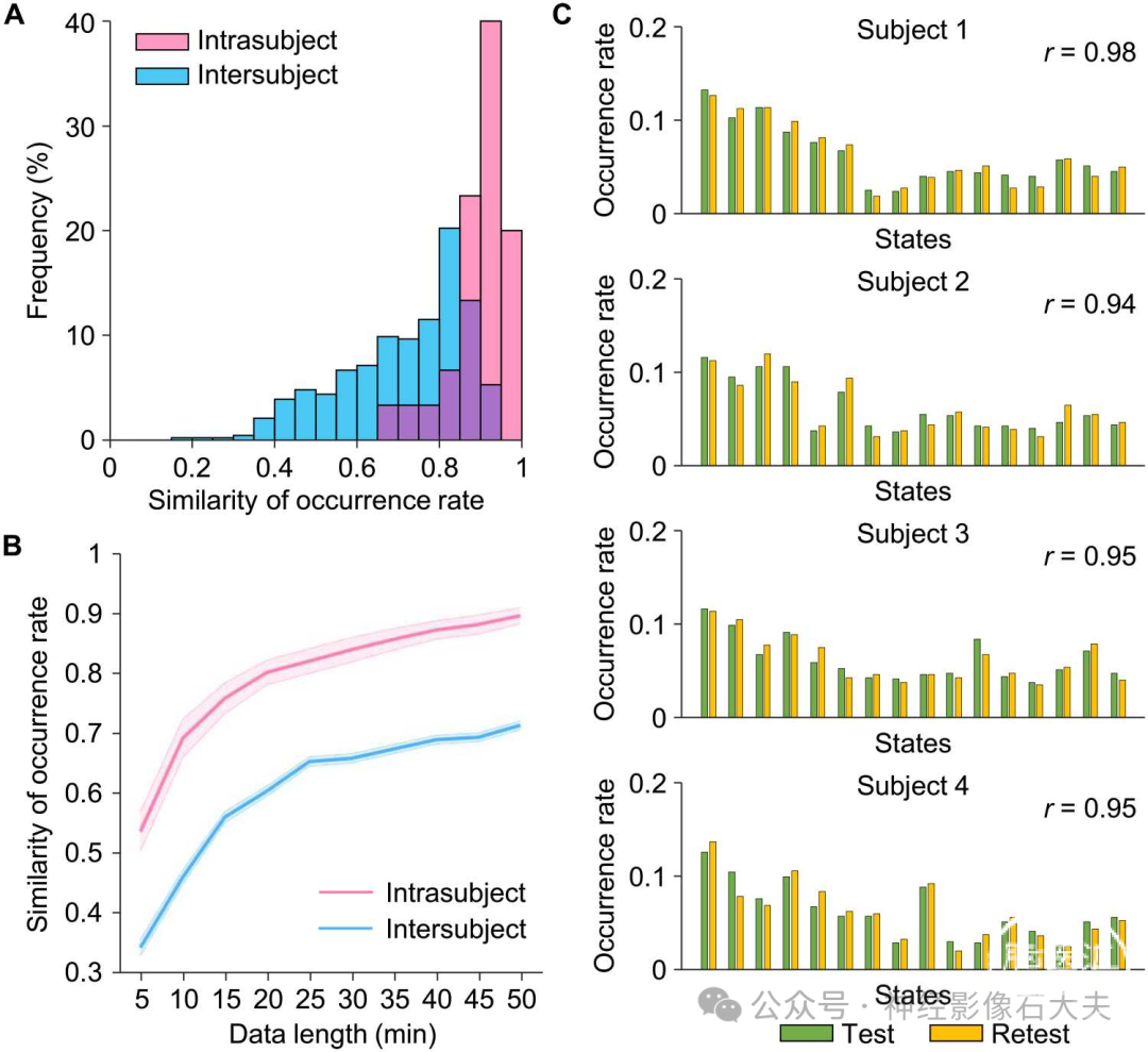
Fig. 3. Estimation of the reliability of the INSCAPE analysis. (A) Test-retest reliability was evaluated using the CoRR-HNU dataset (i.e., Dataset II). We divided each subject’s data equally into two 50-min sessions and calculated the occurrence rates for each session. The intra- and intersubject similarities were quantified by estimating the correlation coefficient of occurrence rates within the same subject and between any two individuals. Correlation analyses yielded a mean intrasubject similarity of r = 0.90 and a mean intersubject similarity of r = 0.71. The frequency distributions of occurrence rates are depicted in a histogram with intrasubject and intersubject similarity denoted by pink bars and blue bars, respectively. (B) The intrasubject (pink line) and intersubject (blue line) similarities in occurrence rates were also examined using the test-retest dataset with 10 different data lengths ranging from 5 to 50 min in duration, in 5-min time increments (mean intrasubject test-retest reliability ± SEM, 5 min: 0.54 ± 0.03, 10 min: 0.69 ± 0.03, 15 min: 0.76 ± 0.03, 20 min: 0.80 ± 0.02, 25 min: 0.82 ± 0.02, 30 min: 0.84 ± 0.02, 35 min: 0.86 ± 0.02, 40 min: 0.87 ± 0.02, 45 min: 0.88 ± 0.02, 50 min: 0.90 ± 0.01). The shaded areas in the figure represent the standard errors. (C) Histograms showing the distributions of test-retest occurrence rates for the 16 brain states extracted from four randomly selected individuals taken from the CoRR-HNU dataset. Green bars represent the occurrence rate of brain states in the test session, while yellow bars represent the occurrence rate of brain states in the retest session.
Brain lateralization is reflected in the network dynamics of coactivated brain states
大脑偏侧化是人类大脑的一个组织原则,被认为有助于快速高效的信息处理。为了辨别16个共激活大脑状态在功能上的偏侧化程度,我们通过比较左右半球之间的激活顶点数量计算了偏侧化指数(LI)。在我们对数据集I的INSCAPE分析得出的16个大脑状态中,状态15和状态11分别显示出最强的左偏侧化和右偏侧化(fig.S4)。左偏侧化状态15的共激活大脑区域包括左侧外侧前额叶皮层、颞顶交界处和后扣带皮层(Fig.4A 和 fig.S5)。右偏侧化状态11在岛叶、角回和背侧前扣带皮层显示出强烈的共激活。此外,我们通过在MNI152体积空间中的小脑掩码内平均相应的原始共激活图,检查了这些偏侧化大脑状态在小脑中的激活模式。大脑中的左偏侧化状态15和右偏侧化状态11在小脑的对侧显示出不对称的功能激活(Fig.4A)。

Fig. S4. Lateralized brain states were selected according to the lateralization index between the left and right hemispheres. The mean coactivation maps of 16 brain states were projected to a FreeSurfer symmetric cortical inflated surface template, consisting of 2,562 vertices per hemisphere. The lateralization index was defined as the difference in the number of activated vertices between the left and right hemispheres divided by the total number of vertices in a given hemisphere. The lateralization indices of the 16 brain states were plotted with positive values indicating left-lateralization and negative values indicating right-lateralization. State 15 showed the highest lateralization index and therefore was selected as the left-lateralized brain state, while state 11 showed the lowest lateralization index and was chosen as the right-lateralized brain state. The mean coactivation maps of the left- and right-lateralized brain states 15 and 11, respectively, are shown in the bottom panel.
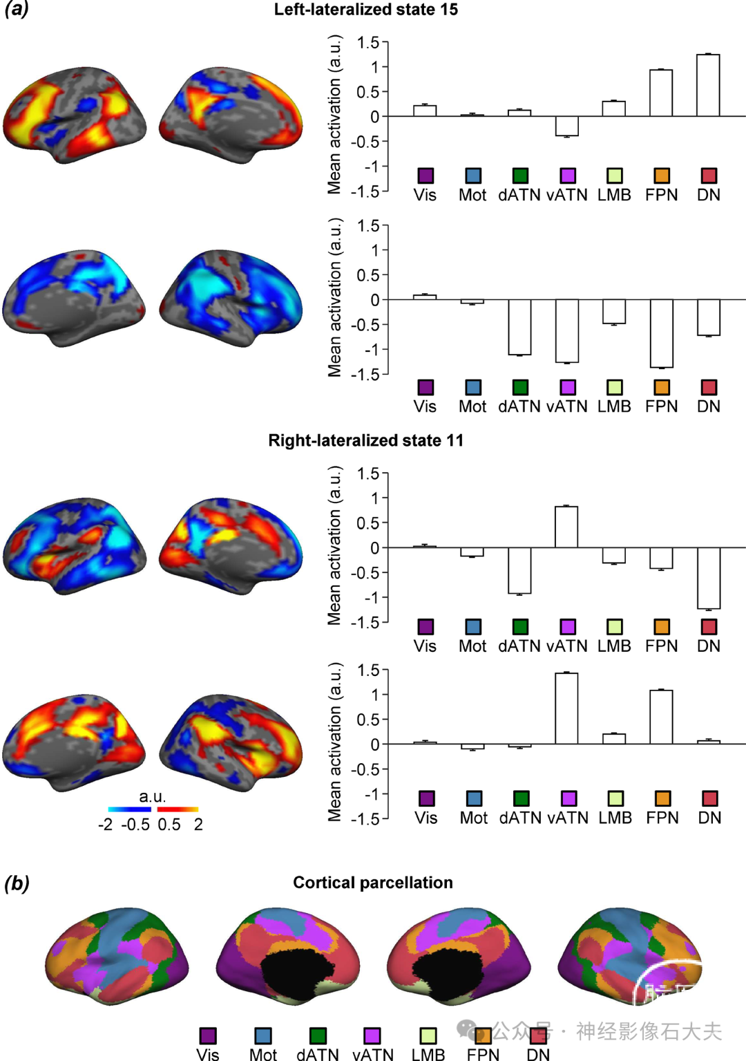
Fig. S5. Lateralization of brain states was quantified across seven canonical cerebral networks in each hemisphere. The mean coactivation maps of left-lateralized state 15 and right-lateralized state 11 were compared with the 7-network cortical parcellation previously employed by Yeo et al (4). (a) The mean coactivation maps for left-lateralized brain state 15 (top panel) and right-lateralized brain state 11 (bottom panel) are shown along side bar graphs displaying the mean coactivations (±SEM) averaged within each of the 7 networks for the left and right hemisphere. (b) The 7-network cortical parcellations projected onto the medial and lateral cortical surface of the left and right hemispheres, which are color-coded to denote network classification. The 7 networks included the visual network (Vis; purple), somatomotor network (Mot; blue), the dorsal (dATN; green) and ventral (vATN; violet) attention networks, limbic network (LMB; cream),frontoparietal control network (FPN; orange) and default mode network (DN; red). Note that left-lateralized state 15 showed the strongest activation in DN and FPN in the left hemisphere and deactivation in FPN, vATN, and dATN in the right hemisphere. Right-lateralized state 11 demonstrated the greatest activation in the vATN bilaterally and in the right FPN, whereas deactivation in DN and dATN in the left hemisphere was observed.
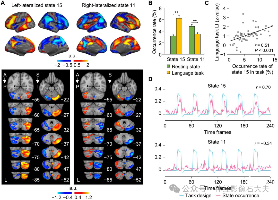
Fig. 4. Cerebral lateralization of coactivated brain states is reflected in the contralateral cerebellum and in language task. (A) Left-lateralized state 15 showed activation in the DN and FPN, as well as cortical areas known to be important for language processing, while activation of right-lateralized state 11 comprised cortical regions anchored in the SN and ventral attention networks. Both lateralized brain states 15 and 11 showed the strongest coactivations in the contralateral cerebellar hemisphere. (B) The occurrence rates of left-lateralized state 15 and right-lateralized state 11 were calculated during resting state and during a language task. Bar graphs depict mean (±SEM) occurrence rates for both states 15 and 11 during resting state (green bars) and the language task (yellow bars). The occurrence of left-lateralized state 15 was significantly greater during the language task compared to resting state, whereas right-lateralized state 11 showed an opposite pattern. (C) Task-based language LI was significantly correlated with the occurrence rate of left-lateralized state 15 in 55 subjects. (D) The occurrence of left-lateralized state 15 was significantly correlated with language task onsets (r = 0.70, P < 0.001), indicating that coactivated regions comprising left-lateralized brain state 15 may subserve language processing. In contrast, the occurrence of right-lateralized state 11 showed a significant negative correlation with task onsets (r = -0.34, P < 0.001).
另一个重要发现是,左偏侧化大脑状态15的共激活区域与传统语言皮层区域高度重叠。为了研究偏侧化大脑状态在多大程度上反映了语言偏侧化的程度,我们估计了55名健康参与者在静息状态和语言任务(即语义决策任务)期间扫描的独立样本(数据集III)中大脑状态15和11的发生率。左偏侧化状态15在语言任务期间的发生率显著高于静息状态[Fig.4B;配对t检验,t(54) = 6.633,**P < 0.001],而右偏侧化状态11在静息状态期间的发生率显著高于语言任务[配对t检验,t(54) = 3.875,**P < 0.001]。然后,我们基于任务诱发的两半球不对称激活计算了每个受试者的基于任务的语言LI。语言偏侧化与任务期间左偏侧化状态15的发生率显著相关(Fig.4C;r = 0.51,P < 0.001)。我们还检查了所有参与者在语言任务每个时间点的大脑状态发生率与任务处理引发的血流动力学响应曲线之间的关系。结果显示,左偏侧化状态15的发生率与语言任务开始时间呈强正相关(Fig.4D;r = 0.70,P < 0.001),而右偏侧化状态11的发生率与语言任务开始时间呈中度负相关(r = -0.34,P < 0.001)。大脑状态9也与语言任务开始时间呈强正相关(fig. S6;r = 0.78,P < 0.001)。基于这些发现,我们将状态15和状态9合并为一个与语言相关的大脑状态,并检查其发生率与语言任务开始时间的关系。我们发现,合并大脑状态的发生率与语言任务开始时间的关联比之前单独观察到的状态15或状态9更强(r = 0.86,P < 0.001)。这些结果表明,左偏侧化状态15和状态9可能在共同支持语言相关的语义处理中协同作用。
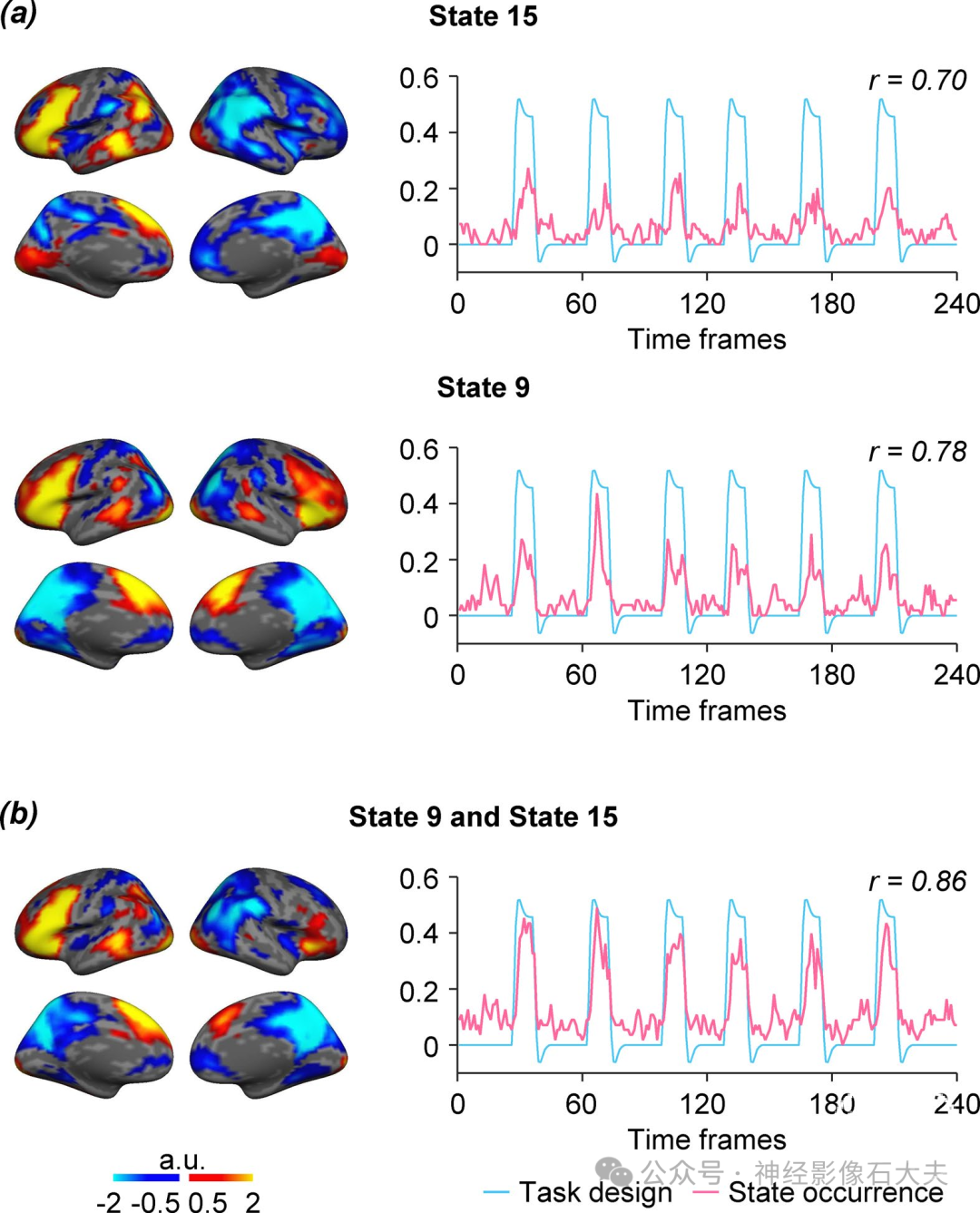
Fig. S6. The occurrence of task-related brain states was frequently coincident with task onset. (a) The occurrence rate of the 16 brain states was quantified in the language task dataset (Dataset III), which contained 55 healthy, adult subjects. The occurrence of each brain state was calculated across subjects at each time point during the language task to generate an occurrence curve of each brain state. Then the state occurrence curve was compared with the hemodynamic response curves of task onsets. The brain state 15 and state 9 showed significant correlation with the task onsets indicating these two states might be involved in the language task processing (Pearson correlation, state 15: r = 0.70, p < 0.001, state 9: r = 0.78, p < 0.001). (b) The brain state 9 and state 15 were then combined as a language-related brain state to calculate its mean coactivation maps and state occurrence curve. The combined brain state has activations in the traditional language areas. The occurrence curve of this combined state is significantly correlated with the hemodynamic response curves of language task onsets (Pearson correlation, r = 0.86, p < 0.001).
最后,鉴于利手和性别对语言功能偏侧化的已知影响,我们在两个独立的数据集中研究了这些表型特征对共激活大脑状态偏侧化的影响。对于利手比较,我们计算了数据集IV中52名左利手和52名人口统计学匹配的右利手受试者中偏侧化大脑状态的发生率。与左利手相比,右利手受试者在右偏侧化状态11中的发生率显著更高[Fig.5A;双样本t检验,t(102) = 2.037,**P = 0.044]。发生率分布还显示,右利手受试者在状态11中的发生率高于左利手受试者(Kolmogorov-Smirnov检验,P = 0.021)。然后,我们检查了数据集V中279名男性和279名人口统计学(匹配年龄、教育和利手)匹配的女性中偏侧化大脑状态发生率的差异。总体而言,男性与女性相比,右偏侧化状态11的发生率显著更高[双样本t检验,t(556) = 2.674,**P = 0.008],并且在左偏侧化状态15中的发生率也显示出显著更高的趋势[Fig.5B;双样本t检验,t(556) = 1.877,P = 0.061]。男性状态11的发生率分布与女性相比显著不同(Kolmogorov-Smirnov检验,P = 0.017),男性在状态11中的发生率相对女性更高。此外,我们研究了利手或性别是否影响状态9的发生率;然而,无论是利手[配对t检验,t(51) = 0.045,P = 0.965]还是性别[配对t检验,t(278) = 0.807,P = 0.420],均未发现显著差异(fig.S7)。
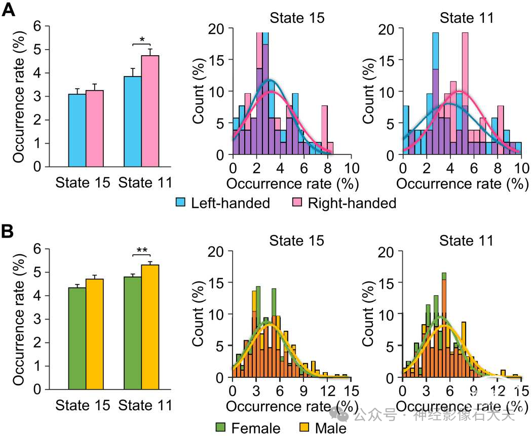
Fig. 5. The influence of handedness and gender on the occurrence rates of lateralized brain states. (A) The occurrence rate of lateralized brain states was computed in 52 left-handed and 52 demographically matched right-handed subjects. Right-handed subjects showed a significantly higher occurrence rate in rightlateralized state 11 relative to left-handers (two-sample t test, *P = 0.044). The occurrence rate distributions for lateralized states 15 and 11 are displayed in the histograms with left-handed subjects depicted by blue bars and right-handed subjects denoted by pink bars, with the overlap of the two shown in purple. The distributions were fitted using Gaussian curves and demonstrate that righthanded subjects showed a higher occurrence rate in state 11 than left-handed subjects (Kolmogorov-Smirnov test, P = 0.021). (B) Occurrence rate of lateralized brain states 15 and 11 across 279 males and 279 matched females. Bar graph depicts the mean percentage of occurrence (±SEM) of states 15 and 11 in male (yellow bars) and female (green bars) subjects. Males demonstrated a significantly higher occurrence of state 11 (two-sample t test, **P = 0.008) and a trend toward a higher occurrence rate in state 15 that approached significance (paired t test, P = 0.054) compared to females. The occurrence rate distributions for these two states are graphically displayed and demonstrate that males (yellow bars) showed a significantly higher occurrence rate in right-lateralized state 11 than females (green bars) (Kolmogorov-Smirnov test, P = 0.017).
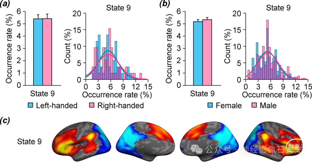
Fig. S7. Language-related brain state 9 is not affected by handedness and gender. In addition to left-lateralized brain state 15, our findings also indicated that brain state 9 was involved in language-related processing. We therefore examined the influence of handedness and gender on the occurrence of brain state 9. (a) The mean occurrence rate (±SEM) of brain state 9 was estimated in 52 left-handed (blue bars) and 52 demographically matched right-handed (pink bars) subjects taken from Dataset IV. No difference was found between leftand right-handed subjects (paired t-test, p = 0.965). The occurrence rate distributions for state 9 are depicted in a histogram denoting left-handed by blue bars and right-handed subjects by pink bars, with the overlap shown in purple. Gaussian curves fit the distributions, demonstrating no difference between left- and righthanded subjects (Kolmogorov-Smirnov test, p = 0.858). (b) The mean occurrence rates of brain state 9 (±SEM) in 279 males (pink bars) and 279 demographically matched females (blue bars). No difference was found between males and females (paired t-test, p = 0.420). The occurrence rate distributions of state 9 are displayed in female (blue bars) and male (pink bars) subjects demonstrates no difference in occurrence rate distributions (Kolmogorov-Smirnov test, p = 0.523). (c) Mean coactivation map for state 9 from the group template projected onto the medial and lateral inflated cortical surface of the left and right hemisphere.
The occurrence rate of dynamic coactivated brain states for assessment of poststroke recovery
个体化的动态大脑状态可用于评估各种脑疾病患者的功能大脑状态,特别是在监测疾病进展或治疗后的恢复过程中。作为概念验证,我们将INSCAPE方法应用于包含42名皮质下卒中患者和23名健康对照参与者的数据集(数据集VI),以评估6个月内的功能变化。我们选择该卒中数据集是因为患者的病因明确且功能损伤在受试者中具有同质性。在卒中后6个月内的五个时间点(即卒中后1至7天、14天、30天、90天和180天)估计了患者中16个大脑状态的发生率。我们还在健康对照组中估计了16个大脑状态的发生率,作为与患者组在卒中后1至7天时间点进行比较的基线。重复测量方差分析(ANOVA)的结果显示,时间有主效应[F(4) = 4.451,P = 0.002,家庭误差率(FWER)校正]。总体而言,在卒中后6个月的恢复期内,患者中左偏侧化大脑状态15的发生率逐渐持续下降。一系列事后配对样本t检验显示,与基线(1至7天)卒中后时间点相比,大脑状态15的发生率在90天[t(41) = 3.662,**P < 0.001]和180天[t(41) = 2.684,*P = 0.01]时显著降低(FWER校正)。急性期状态15的初始升高发生率随时间正常化,并在6个月时与健康对照组相似[双样本t检验,卒中后1至7天:t(63) = 1.883,P = 0.064,卒中后6个月:t(63) = 0.296,P = 0.768]。然而,状态15的发生率与运动评分无直接相关性(P > 0.05)。
鉴于大脑状态15是一个偏侧化的大脑状态,我们假设在卒中后6个月内该状态发生率的持续下降可能表明皮质下卒中导致的半球间对应缺陷的功能逐渐恢复。为了验证这一假设,我们选择了卒中后1至7天时在状态15中激活最高的五个左半球脑区(L1:感觉运动区,L2:顶上小叶,L3:外侧前额叶皮层,L4:颞中回,L5:角回)和五个对称的右半球脑区(R1,R2,R3,R4,R5)(Fig.6B)。计算每对脑区(即L1-R1,L2-R2,L3-R3,L4-R4,L5-R5)之间的功能连接(FC),并在卒中后五个时间点对患者进行平均,以测量半球间连接随时间的变化。重复测量ANOVA的结果表明,时间有显著主效应[F(4) = 4.504,P = 0.002,FWER校正],表明患者在卒中后6个月恢复期内半球间FC逐渐增加(见 fig.S8 中卒中后五个时间点患者每对脑区的FC)。事后配对样本t检验显示,与基线(1至7天)相比,30天[t(41) = 2.201,*P = 0.033]、90天[t(41) = 3.540,**P = 0.001]和180天[t(41) = 2.289,*P = 0.027]时半球间FC显著增加。然后,估计每个半球内任意两个脑区之间的FC并平均以代表半球内连接。在卒中后6个月的恢复期内,患者中两个半球的半球内FC均逐渐下降[重复测量ANOVA,左半球:F(4) = 4.688,P = 0.001,右半球:F(4) = 2.623,P = 0.037]。一系列事后配对样本t检验显示,与急性期相比,90天和180天时两个半球的FC显著降低[卒中后90天与7天相比,左半球:t(41) = 2.874,**P = 0.006,右半球:t(41) = 2.987,**P = 0.005;卒中后180天与7天相比,左半球:t(41) = 2.861,**P = 0.007,右半球:t(41) = 2.456,*P = 0.018]。
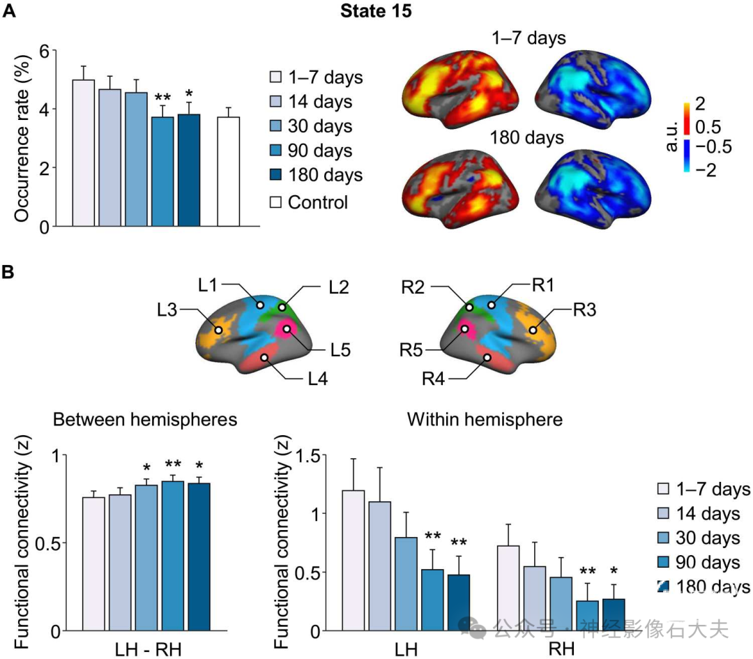
Fig. 6. Longitudinal changes of brain states in patients with subcortical stroke during the first 6 months of recovery. (A) The occurrence rates of the 16 brain states were estimated in patients with subcortical stroke at five time points over a 6-month period (i.e., 1 to 7, 14, 30, 90, and 180 days after stroke). The bar graph shows the mean occurrence rate of state 15 (±SEM) in the patient group (n = 42; blue bars) at each successive time point and in the healthy control group (n = 23; white bars). There was a significant reduction in the occurrence of left-lateralized state 15 in stroke patients at the 90 and 180 days poststroke time points relative to baseline (1 to 7 days after stroke) (paired t test, *P < 0.05 and **P < 0.01). The coactivation maps of left-lateralized brain state 15 in patients at 1 to 7 days and 180 days after stroke are displayed in the right. (B) Five left-hemispheric patches (L1: sensorimotor, L2: superior parietal lobule, L3: lateral prefrontal cortex, L4: middle temporal gyrus, and L5: angular gyrus) that had the highest activations in brain state 15 at the 1 to 7 days poststroke time point and five symmetric right-hemispheric patches (R1, R2, R3, R4, and R5) were selected for the estimation of between- and within-hemisphere connectivity. Between-hemisphere FC increased at the 30, 90, and 180 days poststroke time points relative to baseline (paired t test, *P < 0.05 and **P < 0.01). Both hemispheres showed a gradual reduction in the within-hemisphere connectivity over the 6-month period, and the reduction was statistically significant at 90 and 180 days after stroke compared to the baseline (paired t test, *P < 0.05 and **P < 0.01). LH, left hemisphere; RH, right hemisphere.
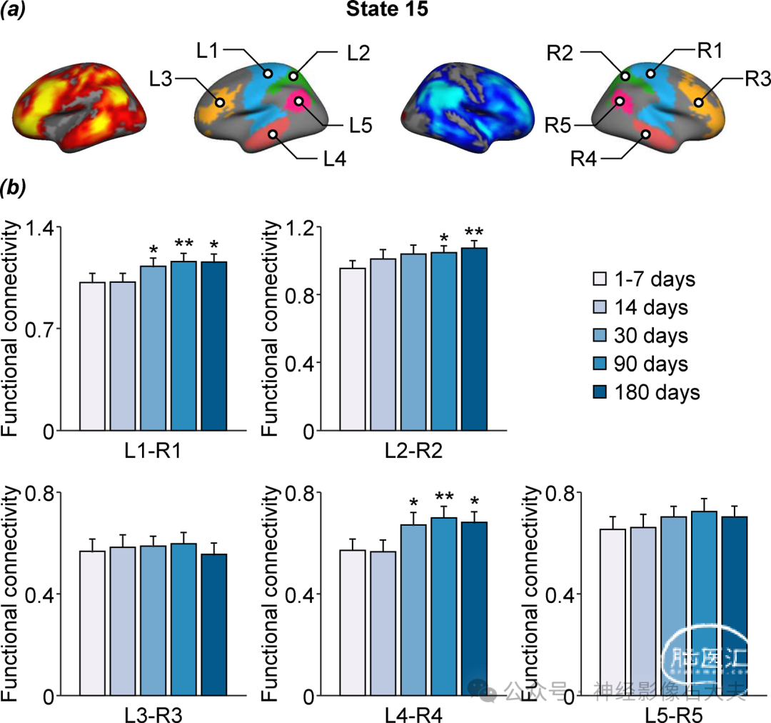
Fig. S8.Between-hemisphere functional connectivity changes in patients with subcortical stroke during the first six months of recovery. (a) The five left-hemispheric patches (L1, L2, L3, L4, and L5) with the highest activations in brain state 15 at the 1-7 day post-stroke time point and the five symmetric patches (R1, R2,R3, R4, and R5) from the right hemisphere were selected as ROIs to evaluate changes in the interhemispheric connectivity at 14, 30, 90 and 180 days post-stroke relative to the baseline time point (1-7 days post-stroke). (b) Static functional connectivity of patch-pairs L1-R1 and L4-R4 showed significant increases over time (repeated-measures ANOVA, p < 0.05) at 30, 90, and 180 days post-stroke compared with baseline (paired t-test, *p < 0.05, **p < 0.01). In addition, static functional connectivity showed a significant increase for the L2-R2 patch pair at 90 and 180 days post-stroke. No significant differences in static functional interhemispheric connectivity for the L3-R3 and L5-R5 patch-pairs across the 5 post-stroke time points were found.
Control analyses
我们将我们的INSCAPE方法与两种先前报道的动态分析方法——Group CAP和HMM-MAR进行了比较。比较在两个独立的数据集中进行——人类连接组计划(HCP)不相关的100名受试者数据集(数据集VII)和CoRR-HNU 30名受试者数据集(数据集II)。我们发现,Group CAP方法在发生率方面的测试-重测可靠性低于INSCAPE和HMM-MAR(见 Supplementary Materials 和 fig. S9)。鉴于HMM-MAR和INSCAPE在发生率方面显示出相似的测试-重测可靠性,这两种方法在空间特征方面进一步进行了比较。我们发现,与HMM-MAR相比,INSCAPE在两个数据集中产生了更稳定的组水平大脑状态(见 Supplementary Materials 和 fig. S10 和 S11)。由于HMM-MAR方法无法在不同数据集中捕捉稳定的群体水平大脑状态,因此从一个数据集中得出的发现可能不容易推广到另一个数据集。我们还发现,INSCAPE在计算上比其他两种方法更高效,使其更容易在大数据样本中使用(见 Supplementary Materials 和 fig. S12)。最后,我们进行了控制分析,以检查头部运动如何影响我们的结果。我们发现,当头部运动不过度时,我们仍然可以解码具有相对可靠的时间和空间特征的大脑状态(fig.S13)。
Discussion
在本研究中,我们利用INSCAPE方法来估计个体水平上的动态功能脑状态。我们证明了使用我们的方法识别的16种脑状态的出现率在个体内具有高度的重测可靠性,同时也捕捉到了显著的个体间差异。我们在不同的实验背景和不同受试者群体中回顾性地应用了这种方法,以开始描述这些特定于个体的脑状态的时空动态特征。我们还发现,一部分表现出功能偏侧化的瞬态脑状态与特定于个体的表型特征(如利手和性别)相关。最后,我们展示了INSCAPE方法可以用于研究神经或精神疾病患者在大规模网络动态中的纵向变化。总的来说,这些发现表明,我们的INSCAPE方法能够稳健且可靠地检测个体水平上的脑状态的动态网络特性,并具有用于研究各种脑疾病的神经和精神后遗症的潜力。
Revealing individual variability in dynamic brain states
复杂、自组织的非线性生物系统(如人脑)的特点是能够快速、适应性地响应外部需求,从而提高生存能力。网络动力学这一新兴的跨学科领域,植根于信息理论和网络科学,旨在综合来自实证和计算研究的综合数据,以更好地理解神经网络动态的时空模式如何随时间展开,并支持在内在静息状态和任务诱导扰动期间的高阶认知过程。先前的研究表明,动态脑网络重构包含了人类认知和行为关键方面的丰富信息,并且还可以反映各种精神疾病和神经疾病中的异常变化。然而,大多数动态FC研究仍然在组水平上进行。研究人类动态脑状态中的个体间差异需要能够捕捉可靠瞬时(moment-to-moment)动态网络重构的成像技术,这些重构在个体水平上快速演变并随时间差异表达。十多年来,滑动窗口方法被广泛用于分析FC模式的内在时间波动。然而,这种方法的时间分辨率有限,因此只能检测到窗口期内的平均状态,这种方法可能会受到已知影响二阶统计的采样变异性的干扰。最近,Janes及其同事提出了一种基于静息态fMRI数据的共激活模式捕捉这些瞬态功能网络重构的方法,并能够在组水平上获得可靠的结果;然而,个体间差异尚未得到评估。在本研究中,我们证明了从我们的INSCAPE方法中得出的脑状态出现率在同一个体内部具有高度可靠性,同时也足够敏感,能够稳健地捕捉个体间的差异(Fig.3)。通过我们的方法描绘这些网络动态大脑状态重构的瞬间变化,可能会为发现有意义的生物标志物以追踪认知能力或疾病状态随时间的变化提供新的研究途径,因为这种方法在检测行为、生理或遗传相关性方面具有更大的统计功效。
Quantitative assessment of brain asymmetry
由于半球偏侧化是人类大脑功能的一个基本组织原则,被认为有助于快速高效的信息处理,因此对其进行了广泛的研究。尽管在使用静态FC指标理解内在大规模网络的功能性大脑偏侧化方面取得了进展,但使用动态FC框架进行的研究相对较少。本研究的一个有趣发现是,两种动态状态可能与大脑功能偏侧化有关。强烈左偏的状态15似乎涉及传统的语言区域,包括额下回、颞上回、顶下小叶和辅助运动区。然而,这种状态也涉及一些DN网络区,如后扣带回。在一个语言任务实验中,这种状态的发生与语言任务的开始显著相关。此外,个体在该状态发生率上的差异可能预测在任务功fMRI期间观察到的语言偏侧化的个体差异(Fig.4)。这些发现表明,状态15可能对语言处理至关重要。相比之下,强烈右偏的状态11似乎涉及传统的注意力区域,包括岛叶和角回。此外,这种状态还涉及一些FPN网络区。这种状态在男性中比女性中更频繁出现,在右撇子中比左撇子中更频繁出现(Fig.5)。先前的研究表明,注意力网络的偏侧化存在利手效应和性别效应。我们推测,状态11可能在注意力处理过程中被激活。
在健康个体以及被诊断患有各种精神疾病和神经疾病的临床人群中,静息状态以及各种认知任务期间的半球不对称性并非静止不变,而是会随着时间推移而发生变化。研究健康个体中大规模网络之间以及内部的功能不对称性的瞬间时空动态变化,可能会增进我们对众多改变大脑偏侧化的神经性疾病的病理生理学的理解。在本研究中,我们发现左偏状态15在中风初期的发生率较高,随后逐渐降低至健康对照组水平(Fig.6)。有观点认为,大脑偏侧化在人类大脑中出现是为了减少半球间交互作用,这可以降低连接成本并提高信息处理效率。因此,中风发作后左偏状态15发生率增加的一种可能解释是,皮质下中风损害了半球间的通信,导致作为功能代偿的皮层偏侧化增强。随着功能恢复,这种代偿效应逐渐减弱。
总的来说,可靠的个体特定的大脑状态可以用来量化个体在偏侧化方面的差异,以及这些差异可能如何与临床症状或认知能力相关。这种方法尤其适合于监测像中风、痴呆和自闭症这类慢性疾病中的大脑实时变化。
Intrinsic and task-induced coactivated brain states share common large-scale network configurations
关于内在静态FC和任务诱导的脑网络变化的研究极大地促进了我们目前对脑网络动态的理解。然而,迄今为止,很少有研究关注自发和任务诱导活动期间出现的网络交互作用和时空动态关系。先前的研究报告称,静息时显示内在FC的区域在任务期间往往会共激活。内在FC揭示的网络架构也存在于各种任务诱导状态中。此外,基于个体受试者任务fMRI数据时间序列的FC网络分割与静息态数据得出的网络非常相似,这表明自发活动和任务诱导扰动在功能网络配置上具有共同点。一个有争议的领域是,在显著不同的任务特定状态以及静息状态下,功能耦合模式的主导趋势是什么。检查动态瞬态共激活脑状态的时空特征可以为动态脑状态重构的协调和可能的竞争提供新的见解。本研究的发现揭示了在静息状态和语言任务期间偏侧化脑状态的出现率共享共同的脑共激活状态(fig.S6)。左右脑偏侧化状态之间的时间分离进一步得到了特定脑状态与语言任务起始时间锁定的观察结果的支持,而相反的右脑偏侧化脑状态显示出任务诱导的去激活,表明网络脑状态配置的解耦或解散 (Fig. 4, B and D)。识别内在和任务驱动的动态脑状态共享的共同特征,不仅有望阐明这些通过不同网络配置和亚稳态状态的快速和流畅过渡如何展开,还可以阐明动态网络变化在多大程度上是状态依赖和/或特质特定的。此外,虽然脑状态共享的时空特性可以为我们提供关于内在静息和任务驱动状态之间共同点的信息,但它也可以阐明这些大规模瞬态网络动态如何随时间演变并重新配置为特定的脑状态或能量景观,以满足不断增加的任务需求。最后,从我们的INSCAPE方法中得出的这些瞬态动态脑状态的个体特异性时空特性,可能有助于确定特定任务在个体水平上修改特定脑状态的程度,特别是在表现出特定网络脑状态共激活模式缺陷或中断的患者中,并可能促进发现各种非侵入性治疗干预的新个性化靶点。
Implications in clinical brain disorder research
许多影像学研究报告了局部分离和全局整合的大规模网络动态协调的中断,这与各种精神和神经疾病有关。几十年来,这些异常的网络动态时空模式通常通过检查静息态fMRI数据时间序列中不同脑区之间的BOLD信号相关性来研究,也称为“静态”FC。然而,基于时间平稳性假设的相关性无法检测到在更短时间尺度上发生的功能网络重构的快速变化。大量新兴证据表明,精神和情绪障碍,特别是与大规模脑网络中动态网络时空模式的改变有关。例如,Kaiser及其同事报告了低频自发时间变化的动态网络共激活模式与重度抑郁症患者自我报告的抑郁严重程度相关的异常模式。Braun及其同事证明,大规模网络重构的动态灵活性的改变部分与精神分裂症的遗传易感性有关。为了能够在更小的时间尺度上检测网络交互作用,我们的小组最近在精神分裂症患者中进行了组水平单帧共激活方法,并发现与精神病症状严重程度相关的患者脑状态出现率的异常变化。在本研究中,我们观察了皮质下卒中患者动态脑状态的纵向变化。具体来说,这些患者在卒中后几天内表现出强烈的左脑偏侧化状态15,随着时间的推移,这种偏侧化脑状态的出现率逐渐减少到健康对照组的水平(Fig. 6)。这一发现与之前使用另一个独立数据集报告的静态FC研究结果一致。这表明,我们的个体化INSCAPE分析方法不仅能够检测脑疾病急性期脑网络之间动态功能相互作用的变化,还可以用于生成生物标志物,以跟踪各种脑疾病的发展和恢复过程,并在个体水平上为治疗选择提供临床指导。
此外,INSCAPE方法的另一个应用是协助传统的FC分析方法在临床研究人群中检测病灶部位或异常网络配置。数据驱动、无假设的FC分析已广泛用于临床研究,以研究与各种神经疾病相关的脑功能异常。这些研究中的FC分析通常用于检查全脑体素或选择为种子的功能分割之间的连接。然而,随着高场MRI的应用,功能成像采集方法的发展,以及分析技术的进步,功能图像的分辨率越来越高,皮层的功能分区也越来越精细。所有这些进步都导致了可以探索的“种子”数量增加。一方面,这对于研究人员来说可能是有利的,因为他们可以比以前想象的更详细地研究脑疾病的时间和空间细节,但同时也增加了陷入统计陷阱的可能性——多重比较次数的增加导致获得假阳性结果的风险更高。为了解决这个问题,我们的INSCAPE方法可以作为一种预分析方法,通过比较个体水平上给定脑状态的出现率作为生物标志物来识别异常的脑共激活状态,同时保留检测患者与健康人群之间疾病引起差异的敏感性。然后,传统的静态FC分析可以用于进一步研究表现出异常脑状态动态的区域之间的功能对应关系。例如,在本研究中,我们揭示了卒中患者偏侧化脑状态的异常(Fig.6A),然后进一步证明了卒中后恢复期间主要运动区和顶叶上叶的FC变化(Fig.6B and fig.S8)。这些发现表明,与无目标地搜索与疾病严重程度和症状持续时间相关的异常病灶部位相比,这是一种更优的跟踪临床终点的策略。
Limitations and future directions
本研究存在一些技术局限性。首先,脑状态的数量选择有些随意。在本研究中,我们选择了16个聚类解决方案,以最大化从测试和重测数据中得出的脑状态的空间相似性。这一过程可以在一定程度上避免聚类数量选择对脑状态时间特征(即出现率)的影响,这是本研究评估的主要动态指标。结合其他指标(如轮廓系数)可能有助于找到最佳聚类数量,可以在未来进行探索。其次,在本研究中,我们选择出现率作为主要指标,而没有评估其他动态指标(如停留时间和状态转换次数)。我们发现停留时间和转换概率高度依赖于出现率。然而,鉴于我们的方法在个体水平上为每个时间帧提供了脑状态标签,可以轻松得出各种次要动态指标,包括停留时间和转换概率。第三,一些最近的研究表明,单体积MRI数据中观察到的共激活模式可能不能完全归因于静息脑活动的非平稳性,应注意所有时间点,而不是那些被认为包含神经事件的时间点。虽然我们发现从INSCAPE方法中得出的脑状态可以反映语言任务期间的神经事件,但应谨慎解释这些状态。第四,我们像传统的静息态fMRI分析一样对数据进行了带通滤波。一些研究表明,静息态fMRI信号的高频振荡(>0.1 Hz)也编码了有意义的神经信息,尽管它们更容易受到心跳和呼吸引起的生理噪声的影响。因此,未来可能对高频带的时间动态感兴趣。最后,在我们当前的INSCAPE流程中,fMRI数据通过从组水平皮层分区得出的分区置信度进行加权。应考虑功能网络动态拓扑组织的个体间差异。例如,在未来的研究中,组分区模板可以替换为个体化皮层分区。
声明:脑医汇旗下神外资讯、神介资讯、神内资讯、脑医咨询、Ai Brain 所发表内容之知识产权为脑医汇及主办方、原作者等相关权利人所有。